Tutorials

It is worth pointing out that this test case takes up more runtime than the other that is provided for the computation of the non-barotropic configuration, hence, it might be useful to check out this test first if you have not done so.

In this setup, we consider a cold rigidly rotating neutron star described by an equation of state (EOS) of the form:

with the free parameters k1 and Gamma.

The potential Q follows the form (Eq. 38 of Camelio et al., 2019)

The simple example that is given in the git repository looks at a cold, rigidly rotating neutron star. In input parameters can be found at the beginning of kepler.f90 and they are:

• gam (double) –> polytropic index of the cold component
• k1 (double) –> proportionality constant of the cold component
• omg0 (double) –> angular velocity (rigid rotation)
• rhostart (double) –> starting density of the Keplerian curve
• rhoend (double) –> final density for the search, e.g., 7d0*rhon
• verbose (logical parameters) –> determines is output is put on the screen
• filename (character) –> defines where to store the results

After following the outlined installation guide, you can run a first test configuration, but it might be worth reducing the resolution (see the discussion about the general settings to know how to do this). Please remember that, in case you change the grid spacing in ASWNS.f90, you have to recompile the code, afterwards you can run it with

./kepler.x

This will prompt an output in which you see the computation of a sequence of TOV stars, e.g.,

TOV: cycle=           1 surf=        1011 M=   1.9273597635660831      x=   1.0000000000000000      dx=   1.0000000000000000
TOV: cycle=           2 surf=         504 M=   1.9290154365593117      x=   2.0000000000000000      dx= -0.11245266184992331
TOV: cycle=           3 surf=         535 M=   1.9293689630752393      x=   1.8875473381500767      dx= -0.15463603290380235
TOV: cycle=           4 surf=         583 M=   1.9290878086382708      x=   1.7329113052462743      dx=   2.8155619686886402E-002
...

followed by the computation of the rotating configuration

 >    1: max|hden - old hden| = 0.8462E-04
 >    2: max|hden - old hden| = 0.1179E-04
 >    3: max|hden - old hden| = 0.1272E-04
 >    4: max|hden - old hden| = 0.1680E-04
 ...

Once in a while, when the required tolerance is met, you see the final output:

## find_kep: iteration=            1
 gravitivational mass =    1.9406076078197565     
 rest mass            =    2.2703990441460347     
 total entropy        =    0.0000000000000000     
 angular momentum     =   0.53421095941810259     
 equatorial radius    =    5.7849999999999211       =    8.5422992991762108       km
 radii ratio          =   0.98271391529818508     
 equatorial Omega     =    1.0000000000000000E-002
 keplerian Omega      =    6.2028428506061051E-002
 disk mass            =    0.0000000000000000     
 central rho          =    1.7355999999999999E-003
 axial Omega          =    1.0000000000000000E-002
 error flag           =            0

This was simply the first step of the iteration, and you see that the code is continuously increasing the mass and trying to find the maximum mass that you can reach the Kepler limit.

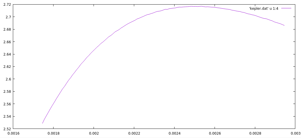
The final results will be written in the file that you provided, by default this would be kepler.dat. The individual columns refer to:

• the central density
• axial Omega
• the corresponding error flag (0 means no error)
• the gravitational mass in Msun
• the baryonic mass in Msun
• the proper mass
• total stellar entropy,
• the angular momentum
• the rotational energy
• the equatorial omega,
• the Keplerian Omega
• the equatorial radius in Msun,
• the equatorial radius in km
• radius at the pole in Msun
• the disk mass
• the derivative dm/drho

Based on the result in kepler.dat, you could check your results. One straight forward way would be to look at m(rho) and plot this with gnuplot, e.g.,

gnuplot gnuplot> plot 'kepler.dat' u 1:4 w l

which gives you the following plot of the gravitational mass as a function of the central density.