Tutorials

For a careful theoretical understanding, one has to investigate the exact model parameters that are employed. The equation of state follows the form (Eq. 45 of Camelio et al., 2019):

with the thermal barotropic law

and the rotational barotropic law (Eq. 24 of Camelio et al., 2019)

with (Eq. 38 of Camelio et al., 2019)

The simple example that is given in the git repository looks at a cold, rigidly rotating neutron star. In input parameters can be found at the beginning of kepler.f90 and they are:

• gam (double) –> polytropic index of the cold component
• gamth (double) –> exponent of the thermal component
• k1 (double) –> proportionality constant of the cold component
• k2 (double) –> proportionality constant of the thermal component
• k3 (double) –> entropy proportionality constant of the barotropic law
• omg0 (double) –> angular velocity in the center
• bvalue (double) –> baroclinic parameter
• rho0 (double) –> central rest mass density
• sigma (double) –> inverse scale radius of the differential rotation sigma = 1/R0
• verbose (logical) –> determines if output is put on the screen
• logfile (character) –> defines where the extended summary of the results is stored
• binfile (character) –> defined where the stellar profiles are stored
• maxit (integer) –> maximum number of iterations for the Newton-Raphson scheme
• tol (double) –> relative tolerance of the employed Newton-Raphson scheme
• relax_iters (integer) –> relaxation iterations in the force balance equation (Euler) solver
• rhocit (double) –> critical density for the EOS inversion from (p, hden) to (rho, s)
• funmax (double) –> maximal value of the function needed for the EOS inversion from (p, hden) to (rho, s)

After following the outlined installation guide, you can run a first test configuration

./nobarotropic.x

The code starts with computing fist some TOV configurations :

TOV: cycle=           1 surf=        1018 M=   1.9735504772232320      x=   1.0000000000000000      dx=   1.0000000000000000
...
TOV: cycle=          10 surf=         564 M=   1.9749035356660132      x=   1.8010690192672787      dx=  -1.3322676295501878E-015

Then, the computation of the non-barotropic configuration begins.

>    1: max|hden - old hden| = 0.6006E-03
>    2: max|hden - old hden| = 0.2515E-03
...
>  289: max|hden - old hden| = 0.1056E-10
>  290: max|hden - old hden| = 0.9721E-11

Once the final tolerance is reached the code provides the final results:

 gravitivational mass =    2.1513803069681354     
 rest mass            =    2.4938629670750729     
 total entropy        =    4.6204903630233412E+057
 angular momentum     =    1.7588646462604272     
 equatorial radius    =    5.9649999999999173       =    8.8080925357970763       km
 radii ratio          =   0.86923721709974955     
 equatorial Omega     =    2.2104905628246539E-002
 keplerian Omega      =    5.9684702928787442E-002
 disk mass            =    0.0000000000000000     
 central rho          =    1.7355999999999999E-003
 central Omega        =    3.5000000000000003E-002
 error flag           =            0

ASWNS also provides a simple script to transform the binary output (that is by default stored in `star.out') to ascii file format. If you want to do this, please start a python environment and run

from binfile_reader import * 
bin2dat(binstar('star.out'),'star.dat')  

This would create an output file with the name star.dat in which you can see the columns theta, r, rest mass density, pressure, internal energy density, fluid velocity, conformal factor, lapse, ZAMO energy, entropy per baryon, and the temperature.

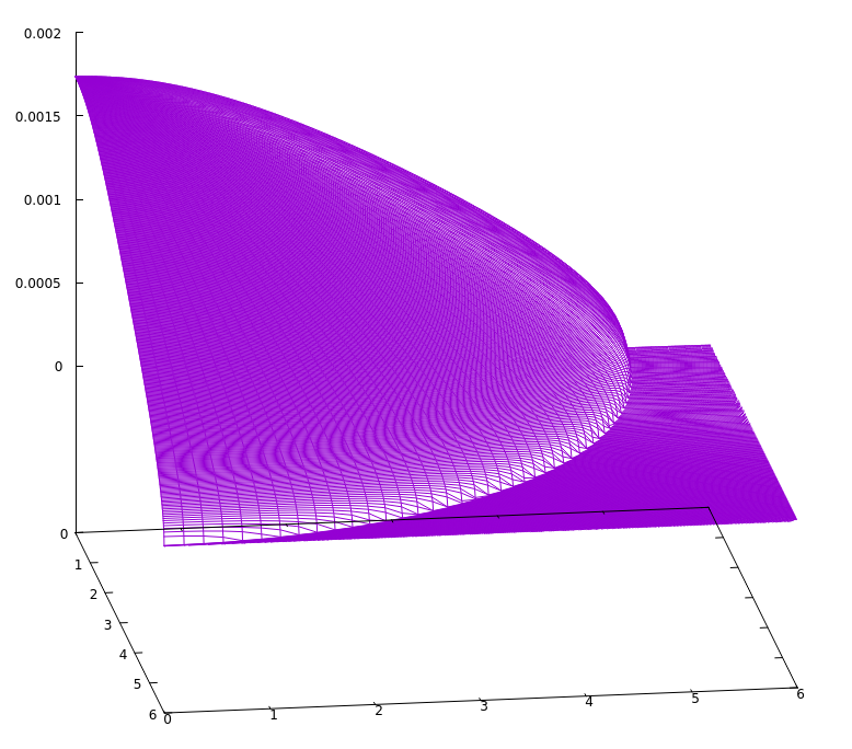
The most straight forward way to make a 2d plot from the data would be to use gnuplot or any other low-level routine and type:

gnuplot 
gnuplot> set xrange [0:10]
gnuplot> set yrange [0:10]
gnuplot> splot 'star.dat' u ($2)*cos($1):($2)*sin($1):($3) w l

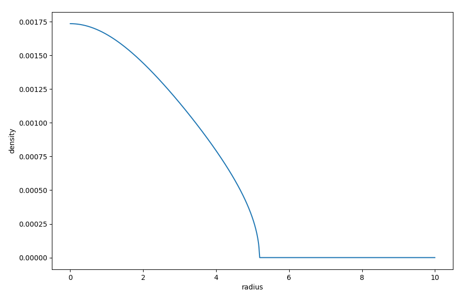
Of course, it would also be possible to produce simple 1d plots and/or use python for plotting, where an example is given below, where we show the density along one radial direction (by using just the first 1000 entries) for approximately theta=0:

import numpy as np
import matplotlib.pyplot as plt

th, r, rho = np.loadtxt('star.dat', usecols=[0,1,2], unpack=True, comments='#')
fig = plt.figure()
plt.plot(r[0:1000], rho[0:1000])
plt.xlabel('radius')
plt.ylabel('density')
plt.show();