This is an old revision of the document!
Light curve inference
NMMA enables to perform parameter estimation in different electromagnetic regimes such as for kilonovae and gamma-ray burst afterglows. Similarly to light curve generation, the following models are available for kilonova inference: Bu2019nsbh (BH-NS model), Bu2019lm (BNS model), Me2017 (BNS model), and Ka2017 (BNS model).
Kilonovae
Example: Me2017 Model
At first, a number of BNS injections based on a specific EOS and prior can be compiled by using:
nmma_create_injection --prior-file priors/Me2017.prior --eos-file example_files/eos/ALF2.dat --binary-type BNS --n-injection 100 --original-parameters --extension json
This generates a file called injection.json that includes an injection file drawn from the prior file with a number of injections specified by –n-injection. The injection file generated for a certain kilonova model, (see also here) can be used to start a Bayesian inference analysis for kilonovae. The Bayesian inference can be started using:
light_curve_analysis --model Me2017 --svd-path ./svdmodels --outdir outdir --label injection --prior priors/Me2017.prior --tmin 0.1 --tmax 20 --dt 0.5 --error-budget 1 --nlive 512 --Ebv-max 0 --injection ./injection.json --injection-num 0 --injection-outfile outdir/lc.csv --generation-seed 42 --filters u,g,r,i,z,y,J,H,K --plot --remove-nondetections
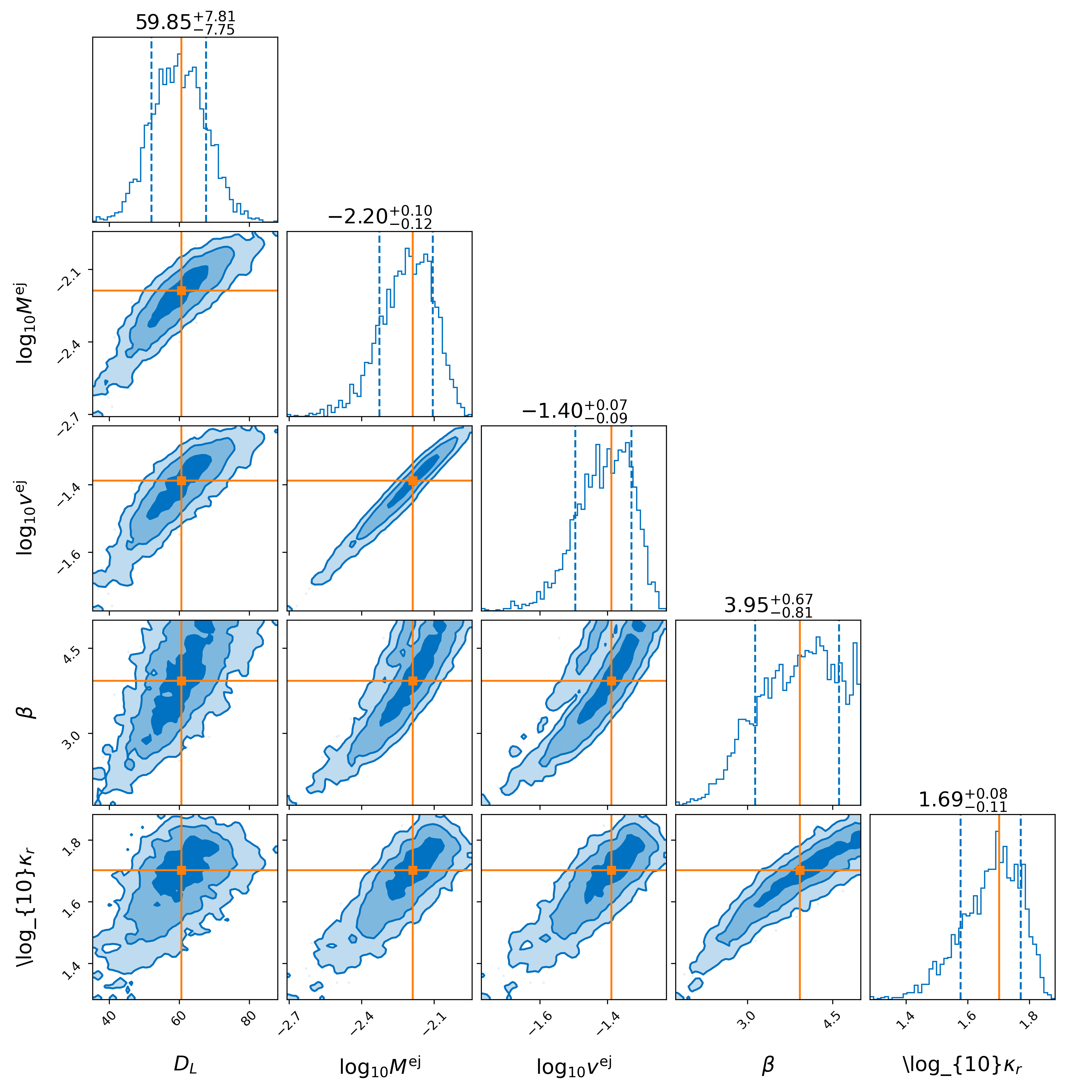
A result of obtained posteriors is shown below:

Example: Bu2019lm Model
In order to perform parameter estimation with observational data, a prior as well as the observational data is required. In this example, we use the Bu2019lm model to perform Bayesian inference on the observed kilonova event AT2017gfo.
Gamma-ray burst afterglows
Example: TrPi2018 Model
