Tutorials

NMMA enables to generate electromagnetic light curves in different electromagnetic regimes. For the light curve generation, the user can select among different models. The current version of NMMA includes three kilonova light curve models and enables to compute Gamma-ray burst afterglow light curves which is based on the model afterglowpy published by [1].

For kilonova light curve generation, the following models are available in NMMA:

• Bu2019nsbh - a BH-NS model,
• Bu2019lm - a BNS model
• Me2017 - a BNS model
• Ka2017 - a BNS model

Note that the parameters vary from model to model - an overview can be found here. Some models such as Bu2019lm require to embed a SVD grid for light curve computation which can be found here. With these, a light curve object can be instantiated as follows:

tmin=0.1
tmax=20.0
deltat=0.1
t = np.arange(tmin, tmax, deltat)
lc_model = nmma.em.model.SVDLightCurveModel(model='Bu2019lm', sample_times = t, svd_path = "nmma/svdmodels/", parameter_conversion=None, mag_ncoeff=None,  lbol_ncoeff=None)

By providing input values for a chosen model, a kilonova light curve in different photometric bands can be generated using:

params_range = {
  'log10_mej_dyn': -3,
  'log10_mej_wind': -3,
  'KNphi': 15,
  'inclination_EM': 0,
  'luminosity_distance': 40}
lbol, mag= lc_model.generate_lightcurve(t, params_range)

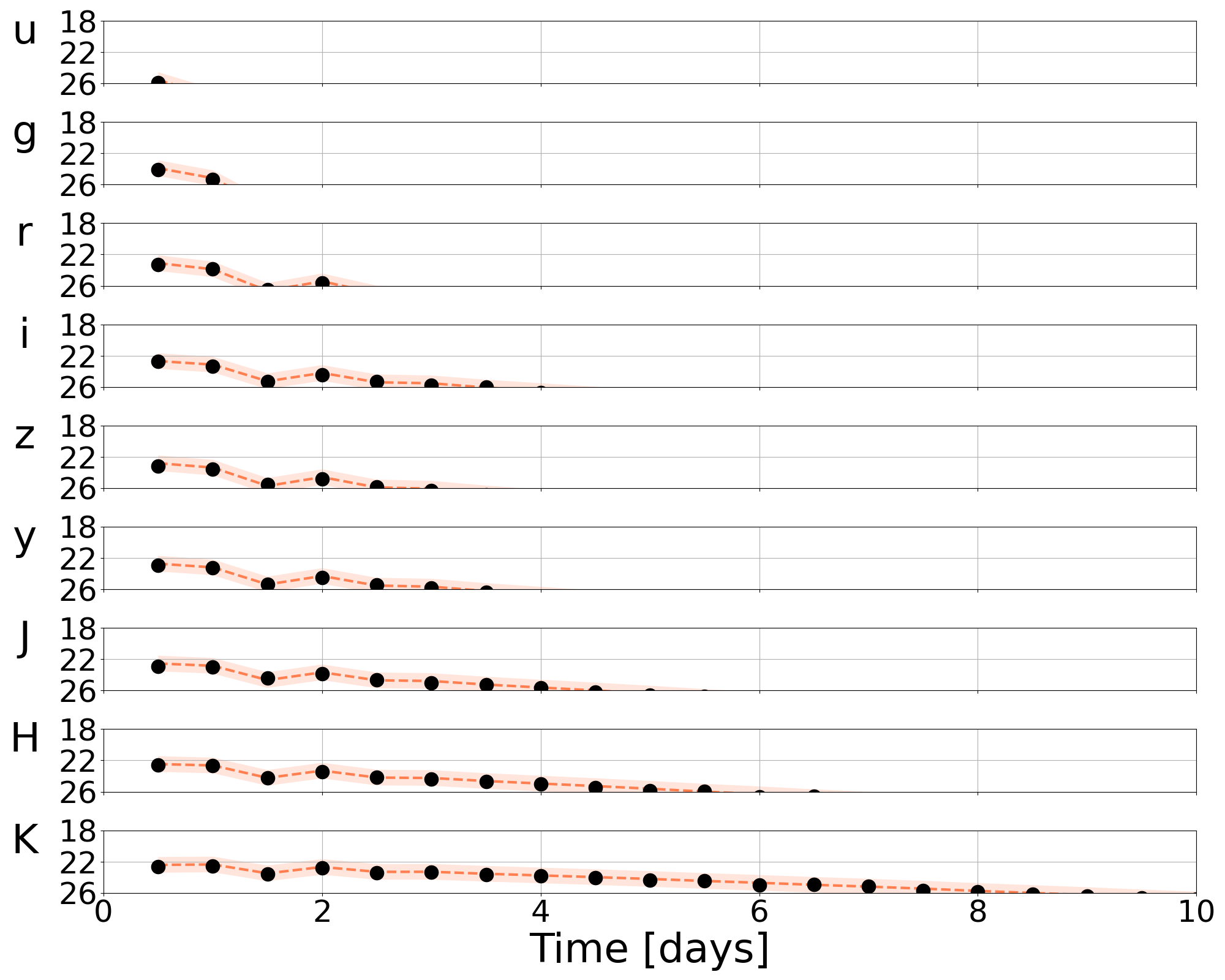
Through the filter keys such as u,g,r,i,z,y,J,H,K, the light curves in different photometric bands can be obtained, e.g., using mag['u']. An example plot of kilonova light curves in different photometric bands is shown below for AT2017gfo.

In order to compute GRB afterglow light curves, NMMA uses the model TrPi2018 from afterglowpy and enables a GRB afterglow light curve generation on a fixed time grid.

import nmma.em.model
t_day = np.arange(1., 950., 1.)
grb_model = nmma.em.model.GRBLightCurveModel(t_day, resolution=12, jetType=0) 
params_range = {
  'inclination_EM': 0,
  'log10_E0': 50.,
  'thetaCore': 0.05,
  'thetaWing': 0.01,
  'log10_n0':-4.5,
  'p':2.160,
  'log10_epsilon_e':-1.6, 
  'log10_epsilon_B':-2.,
  'luminosity_distance': 40,}

lbol, mag = grb_model.generate_lightcurve(t_day, params_range)

GRB afterglow light curves can be accessed with the filter keys X-ray-5keV and X-ray-1keV, e.g. mag_abs['X-ray-5keV'].

NMMA uses a model from Piro et al. 2021. Following a shock breakout, the radiation of shock heated material expands and cools, known as shock cooling emission. The emission in different spectral regimes can be computed as follows:

t = np.arange(tmin=0.1, tmax=10., deltat=0.1)
sn_model = nmma.em.model.ShockCoolingLightCurveModel(sample_times = t, parameter_conversion=None, model="Piro2021")
params_range = {
  'log10_Menv': 30,
  'log10_Renv': 20,
  'log10_Ee': 49.,
  'luminosity_distance': 1.234e+24,}
lbol, mag = sn_model.generate_lightcurve(t, params_range)